Gradient Descent: Under the Hood
At a concrete level, we can walk through the gradient descent steps using a small e-commerce dataset containing five examples, utilizing Mean Squared Error (MSE) as the loss metric, mathematically denoted as \( J(w, b) \):
| Ad Spend in $1000s (feature: \( x \)) | Sales in $1000s (label: \( y \)) |
|---|---|
| 1.00 | 2.0 |
| 2.00 | 4.0 |
| 3.00 | 5.0 |
| 4.00 | 7.0 |
| 5.00 | 9.0 |
Initialize Parameters
The algorithm begins by setting the weight (\( w \)) and bias (\( b \)) to zero:
Where \( \hat{y} \) (y-hat) represents the model’s predicted value.
Calculate Initial Loss
Calculate the MSE loss function, \( J(w, b) \), with the initial parameters against all 5 examples:
Calculate the Gradient (Slope)
Calculate the steepness and direction of the loss function relative to both parameters:
Expand to see calculus derivation
To determine the local slope for the parameter updates, we take the partial derivative of the MSE function with respect to \( w \) and \( b \).
Weight Derivative
The partial derivative of the loss function with respect to the weight (\( w \)):
We compute the error for each example, multiply by its feature value \( x \), sum the results, and scale by \(-2/N\). Substituting \( w=0 \) and \( b=0 \) into this dataset yields: \((-2/5) \times 98 = -39.2\).
Bias Derivative
The partial derivative of the loss function with respect to the bias (\( b \)):
We simply sum the raw errors and scale by \(-2/N\). Substituting the initial zeros yields: \((-2/5) \times 27 = -10.8\).
Update Parameters
Step in the opposite direction of the gradient to descend the error curve. We apply the update rule using a learning rate (\( \alpha \)) of 0.02:
0 - (0.02 × -39.2)
0 - (0.02 × -10.8)
We use the updated weight (\( w = 0.78 \)) and bias (\( b = 0.22 \)) to recalculate the loss and repeat the gradient computation. Projecting this out for six total iterations produces the following convergence trajectory:
| Iteration | Weight (\( w \)) | Bias (\( b \)) | Loss \( J(w,b) \) |
|---|---|---|---|
| 1 | 0.00 | 0.00 | 35.00 |
| 2 | 0.78 | 0.22 | 13.42 |
| 3 | 1.28 | 0.35 | 5.35 |
| 4 | 1.58 | 0.42 | 2.30 |
| 5 | 1.75 | 0.46 | 1.14 |
| 6 | 1.85 | 0.48 | 0.69 |
Deriving the Gradients: The Chain Rule
1. The Setup
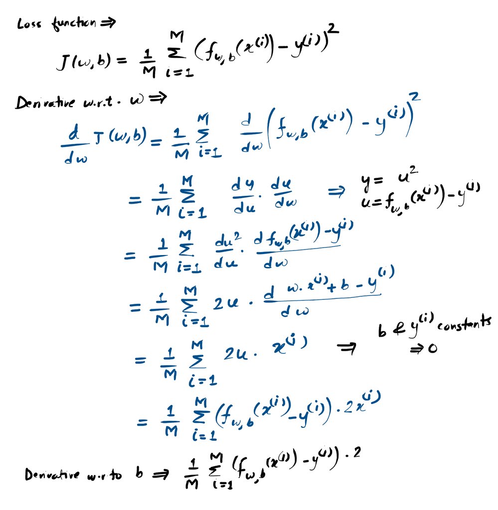
To optimize the model, we must find the partial derivatives of the Mean Squared Error (MSE) loss function with respect to the weight (\( w \)) and the bias (\( b \)). We start with our two foundational equations:
The Chain Rule: Because the linear prediction function is nested inside the squared error function, we take the derivative of the outer function and multiply it by the derivative of the inner function.
2. The Weight Derivative
-
Step A: The Outer Derivative
Treat the inner parenthesis as a single variable (\(u^2\)). Applying the power rule drops the exponent 2 to the front.
\( 2 \cdot (w \cdot x^{(i)} + b – y^{(i)}) \) -
Step B: The Inner Derivative (w.r.t \( w \))
Derive the inside function strictly with respect to \( w \). Constants \( b \) and \( y \) become 0. The derivative of \( wx \) is simply \( x \).
\( \frac{\partial}{\partial w} (w \cdot x^{(i)} + b – y^{(i)}) = \mathbf{x^{(i)}} \) -
Step C: Multiply & Reformat
Multiply Step A by Step B, place it back inside the summation, and swap the prediction notation back in.
\[ \frac{\partial J}{\partial w} = \frac{1}{M} \sum_{i=1}^{M} (f_{w,b}(x^{(i)}) – y^{(i)}) \cdot 2x^{(i)} \]
3. The Bias Derivative
-
Step A: The Outer Derivative
This remains exactly the same as the weight derivative. The exponent 2 drops to the front.
\( 2 \cdot (w \cdot x^{(i)} + b – y^{(i)}) \) -
Step B: The Inner Derivative (w.r.t \( b \))
Derive the inside function strictly with respect to \( b \). The \( wx \) and \( y \) terms are treated as constants (becoming 0). The derivative of a standalone \( b \) is 1.
\( \frac{\partial}{\partial b} (w \cdot x^{(i)} + b – y^{(i)}) = \mathbf{1} \) -
Step C: Multiply & Reformat
Multiply Step A by Step B. Because multiplying by 1 changes nothing, the \( x \) feature vanishes completely from this formula.
\[ \frac{\partial J}{\partial b} = \frac{1}{M} \sum_{i=1}^{M} (f_{w,b}(x^{(i)}) – y^{(i)}) \cdot 2 \]
Reference
-
Google for Developers, 2026.
https://developers.google.com/machine-learning/crash-course/linear-regression/gradient-descent -
Ibm.com, Mar. 27, 2024.
https://community.ibm.com/community/user/ai-datascience/blogs/danish-hasarat/2024/03/26/optimization-understanding-gradient-des -
Github.io.
https://sbu-python-class.github.io/python-science/11-machine-learning/gradient-descent.html -
Mit.edu, 2026.
https://visionbook.mit.edu/gradient_descent.html -
Ibm.com, Dec. 16, 2024.
https://www.ibm.com/think/topics/gradient-descent