The Agent-Environment Interaction
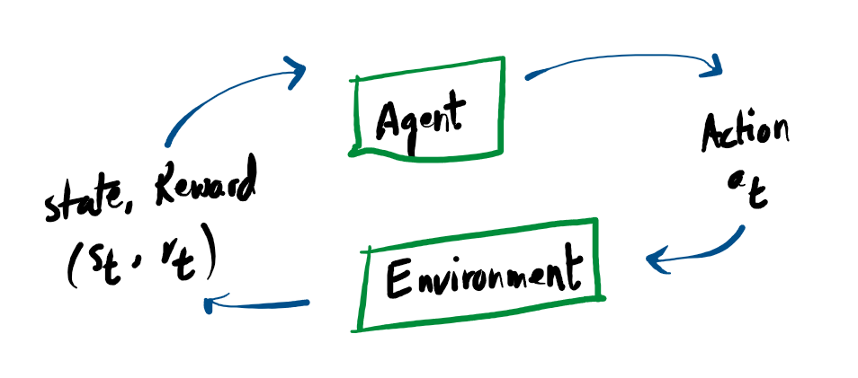
In Reinforcement Learning, the two core components are the Agent and the Environment. The environment serves as the simulated or physical world where the agent operates.
In a continuous loop, the agent receives an observation detailing the current condition of this world. Based on that information, it executes a specific action. The environment then updates and shifts to a new state, driven both by the agent’s action and its own internal rules of physics or logic.
Key Concepts of Reinforcement Learning
Reinforcement Learning (RL) is about an Agent learning to master an Environment through trial, error, and rewards. Here is the absolute shortest breakdown of the core terminology:
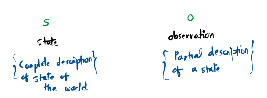
A complete (state) or partial (observation) description of what the environment looks like right now.
What the agent decides to do (e.g., move left, jump, apply torque to a motor).
The immediate points scored (r) vs. the total cumulative score (R). Future rewards are often discounted by γ.
The agent’s “brain” or rulebook. It is a mathematical function that maps a state to a chosen action.
The recorded timeline of a single episode: State → Action → Reward → Next State.
The agent’s prediction of its expected future Return starting from its current state or action.
Interactive RL Loop
Watch how the math flows to build a Trajectory (τ)
States and Observations
A state s provides a comprehensive blueprint of the environment at a specific moment, with absolutely no hidden variables. Conversely, an observation o offers merely a restricted or incomplete view of that state, where certain details remain obscured from the agent.
In the realm of Deep Reinforcement Learning, both states and observations are typically encoded mathematically as real-valued vectors, matrices, or higher-order tensors. To illustrate, a video game agent might process an observation as a dense grid of RGB pixel values, whereas a robotic arm’s state might be defined by a precise array of joint angles and movement speeds.
Environments that grant the agent total access to all underlying variables are known as fully observed. On the other hand, when the agent must make decisions based on restricted sensory input, the system is classified as partially observed.
Action Spaces
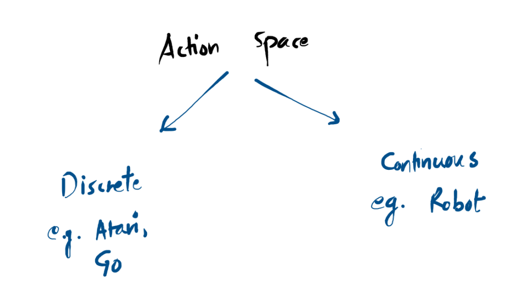
Every environment defines an Action Space the complete menu of valid moves an agent is allowed to make. These spaces generally fall into two distinct categories:
Understanding this distinction is critical in deep reinforcement learning. Many algorithms are mathematically designed to solve only one type of action space, and applying them to the other requires a complete structural rework of the AI’s neural network.
Policies: The Agent’s Brain
A policy is the fundamental rulebook an agent uses to decide which action to take in any given state. Because the policy dictates behavior, researchers often substitute the word “policy” for the “agent” itself.
In Deep Reinforcement Learning, we use parameterized policies. This means the policy is powered by a neural network. The network’s weights and biases are the parameters (denoted as θ), which an optimization algorithm adjusts over time to improve performance.
1. Deterministic Policies
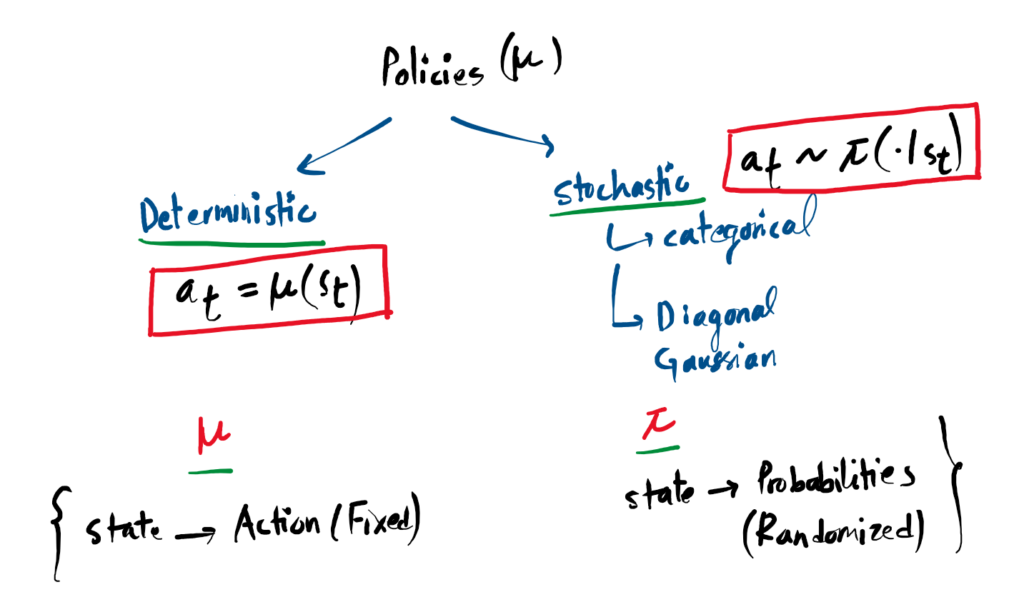
A deterministic policy maps a state directly to one exact, specific action. There is no randomness. If the agent sees the exact same state twice, it will take the exact same action twice. It is usually denoted by the symbol μ:
2. Stochastic Policies
A stochastic policy outputs a probability distribution over a range of possible actions. The agent then rolls the dice and samples an action from that distribution. This randomness is crucial for letting the agent explore its environment. It is denoted by the symbol π:
To train a stochastic policy, algorithms need to do two things: mathematically sample an action, and calculate the Log-Likelihood log πθ(a|s) (how probable that specific action was). There are two main types of stochastic policies depending on the action space:
- Categorical Policies (For Discrete Actions): Works like an image classifier. The neural network outputs probabilities for a finite set of buttons (e.g., 10% Jump, 70% Duck, 20% Punch). The action is sampled based on those percentages.
- Diagonal Gaussian Policies (For Continuous Actions): Works for fluid movements (like steering). The neural network outputs a Mean (μ) and a Standard Deviation (σ). The action is sampled by taking the mean and adding random spherical noise.
Action Sampling Simulation
Click the button to see how different policies react to the exact same environment state.
Always outputs exact center.
Samples discrete choices based on weight.
Samples continuous values around a mean.
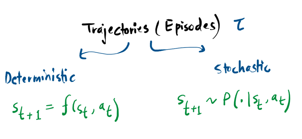
Trajectories (Episodes)
A trajectory τ represents a chronological record of an agent’s experience in the world. It is a sequence consisting of every state encountered and every action taken during a specific period of time:
The journey begins at an initial state s0, which is randomly chosen from a starting distribution ρ0. From there, the sequence evolves through State Transitions.
These transitions the movement from one state to the next are determined by the environment’s internal logic. This transition depends strictly on the most recent state and action. It can be deterministic (the outcome is certain) or stochastic (the outcome involves probability).
While the environment controls the transitions, the actions themselves are provided by the agent according to its specific policy. In Reinforcement Learning literature, these recorded sequences are also commonly referred to as episodes or rollouts.
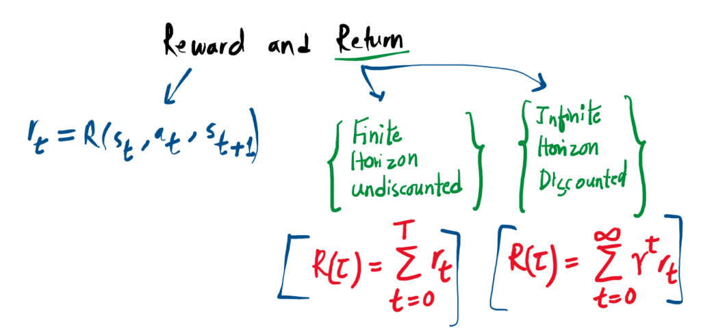
Reward and Return
The reward function is the engine that drives reinforcement learning. It acts as the immediate feedback mechanism, outputting a number that tells the agent exactly how “good” or “bad” its current situation is.
Mathematically, the reward rt often depends on the current state, the action taken, and the resulting next state. However, it is frequently simplified to just depend on the current state-action pair:
The ultimate goal of the agent is not just to get a high reward right now, but to maximize its cumulative reward over time. We call this total accumulated score the Return, denoted by R(τ). There are two standard ways to formulate this Return.
1. Finite-Horizon Undiscounted Return
If an episode has a strict time limit (a fixed window of steps), we can simply add up all the rewards the agent collected before the timer ran out:
2. Infinite-Horizon Discounted Return
If an environment runs forever, simply adding up rewards would result in an infinite sum, breaking the underlying math. To solve this, we introduce a discount factor γ (gamma), a number between 0 and 1.
Why use a discount factor? Intuitively, it mimics real life: a dollar today is worth more to you than a dollar promised ten years from now. The agent prefers immediate rewards over distant, uncertain ones. Mathematically, multiplying future rewards by a fraction (γt) ensures that the infinite sum safely converges to a finite, computable number.
The Discount Factor Simulation
Assume the agent receives a constant reward of +100 at every timestep. Adjust Gamma (γ) to see how it shrinks the value of future rewards.
Notice how a Gamma of 1.0 treats all future rewards equally, while a Gamma of 0.0 makes the agent incredibly short-sighted, completely ignoring everything except the very first immediate reward.
Value Functions & Bellman Equations
While a reward tells the agent how it is doing now, a Value Function predicts how the agent will do over the long haul. It estimates the total future return the agent can expect to receive starting from a specific point.
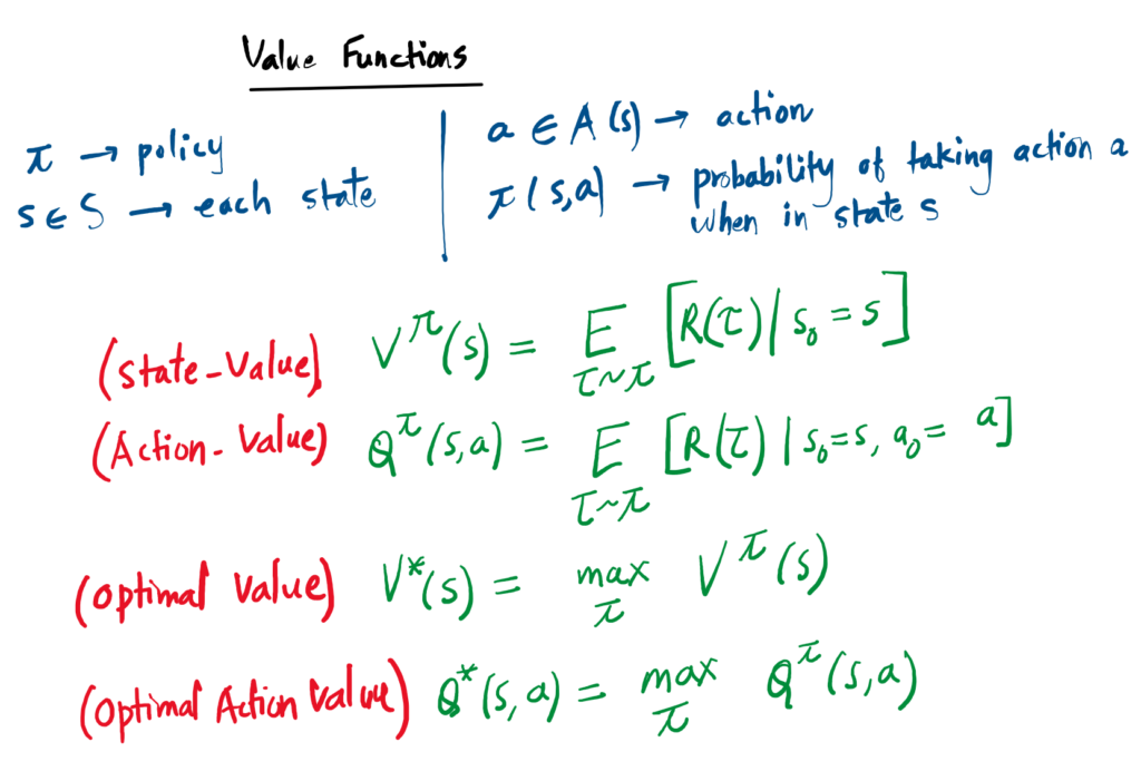
1. The Four Main Functions
In reinforcement learning, we primarily track four types of “expectations”:
- State-Value Vπ(s): Expected return starting in state s following policy π.
- Action-Value Qπ(s,a): Expected return starting in state s, taking action a, then following policy π.
- Optimal Value V*(s): The highest possible return achievable from state s.
- Optimal Action-Value Q*(s,a): The highest possible return starting with action a.
2. Bellman Equations
The “Bellman Equation” is a self-consistency rule. It states that the value of where you are now must equal the reward you just got, plus the discounted value of where you land next.
Value(Now) = Reward + Discounted Value(Next)
3. The Advantage Function
Sometimes we don’t care about the absolute value, but rather how much better one action is compared to the average. This is the Advantage Function Aπ(s,a). It is the difference between the Action-Value and the State-Value:
4. The MDP
The math above is formalized as a Markov Decision Process (MDP). An MDP is defined by a 5-tuple ⟨ S, A, R, P, ρ0 ⟩. It operates on the Markov Property: the future depends only on the current state and action, not the path taken to get there.
Take a Quiz.
References
-
[1]
“Part 1: Key Concepts in RL — Spinning Up documentation,” Openai.com, 2018.
https://spinningup.openai.com/en/latest/spinningup/rl_intro.html -
[2]
J. M. Ph.D and E. Kavlakoglu, “Reinforcement Learning,” Ibm.com, Mar. 25, 2024.
https://www.ibm.com/think/topics/reinforcement-learning - [3]
-
[4]
R. S. Sutton and A. G. Barto, “Reinforcement Learning: An Introduction.” MIT Press.